1 Why Mamba and Structured State Space Sequence Models?
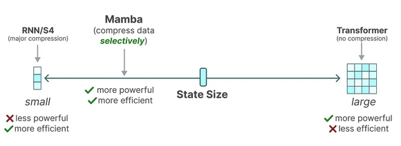
The fundamental problem in deep sequence modelling is how to efficiently compress the context into a smaller learnable state representation whilst maintaining the quality of state representation. As seen in Figure 1.1, transformers have powerful in-context learning capabilties due to the inherent nature of attention but it’s uncompressed memory state (the attention matrix) makes for inefficient inference especially with long-range dependencies (LRD) or large context window settings. On the other end, RNNs and S4 models may be efficient but fail to preserve context state required to perform well in tasks that require in-context reasoning. Mamba proposes a context-aware method to dynamically filter out inputs in the sequence to effectively compress the context.
The Mamba model architecture has recently emerged as a promising alternative to deep sequence modelling overcoming key limitations in other model families such as S4, transformers, recurrent neural networks (RNNs), convolutional neural networks (CNNs), in performing context-aware reasoning with extreme large context windows, up to 1 million tokens.
Structured state space models (SSMs) are particularly useful for modelling long-range dependencies in continuous data such as time series and signal data [2]. It offers a robust framework for handling long-range dependencies efficiently with - up to 5x higher throughput than transformers - linear scaling with sequence length - in-context learning performance improvement on real data up to million-length sequences [3].
Therefore, their strengths are suited to problems that require the ability to process long-range dependencies such as high frame-rate medical signals, speech, video, energy waveforms, DNA sequences and summarising, generating and performing reasoning on novels, movies, and large data corpuses.
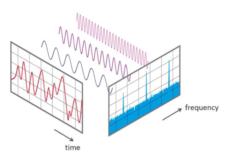
It primarily does this by framing the modelling problem of learning complex non-linear interdependencies between inputs and outputs as a discretised signal-to-signal learning problem. It aims to learn the compressed selective memory state between a higher-dimensional input signal and its online function reconstruction with the goal to compress the properties of the continuous signal in a discrete space. It borrows ideas from control theory and signal processing, where it is analogous to learning an evolving first-order differential equation (eg. Kalman Filter as a state space model) to capture the input signal’s dynamics whilst employing structured matrices (e.g. HIPPO matrix operator [5], diagonal plus low-rank matrices) to reduce computational complexity and utilising Fast Fourier transforms (FFTs) to further speed up computations.
The predecessor to Mamba, the S4 model [6], was the first SSM to show promising results in the Long Range Arena [2] even on the Path-X task where the task is to determine whether two points are connected between a flattened sequence of the image which is notable as many other models fail at this task as seen in Figure 1.3.
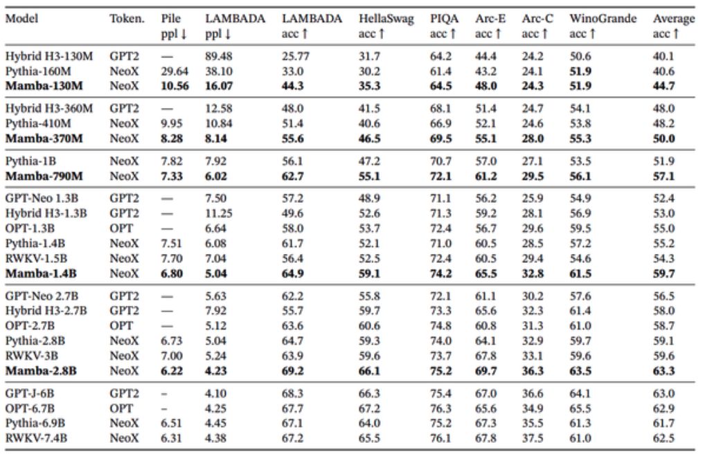
Mamba has also been shown to hold its own against the Transformer++ recipe (eg. PaLM and LLama architectures), eg. linear scaling with sequence length and model parameters via its parallel scan algorithm implementation {Section 3.2.1}. As a general sequence model backbone, Mamba achieves state-of-the-art performance across several modalities such as language, audio, and genomics. On language modelling, the Mamba-3B model outperforms Transformers of the same size and matches Transformers twice its size, both in pretraining and downstream evaluation [3].
1.1 Limitations of Transformers for Long Contexts
In recent years, the transformer architecture has dominated AI, leading to significant advancements in various fields, including solving the protein folding problem (AlphaFold), performing in the 80-90th percentile in the uniform bar exams and college-level AP subjects[7], to translating between nuanced languages from Tamil, Turkish, Arabic to Urdu. However, transformers face challenges with long sequences (e.g., 100,000 tokens or more) due to the quadratic complexity of the self-attention mechanism, which results in substantial computational and memory costs especially during inference due the \(N^2\) size of the \((QK)V\) matrix.
\[ \text{Attention}(Q, K, V) = \text{softmax}\left(\frac{Q K^T}{\sqrt{d_k}}\right) V \tag{1.1}\]
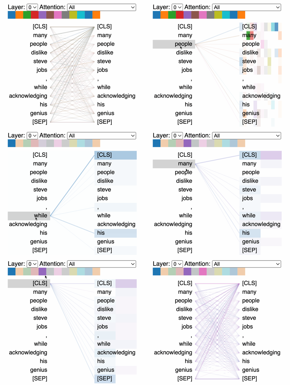
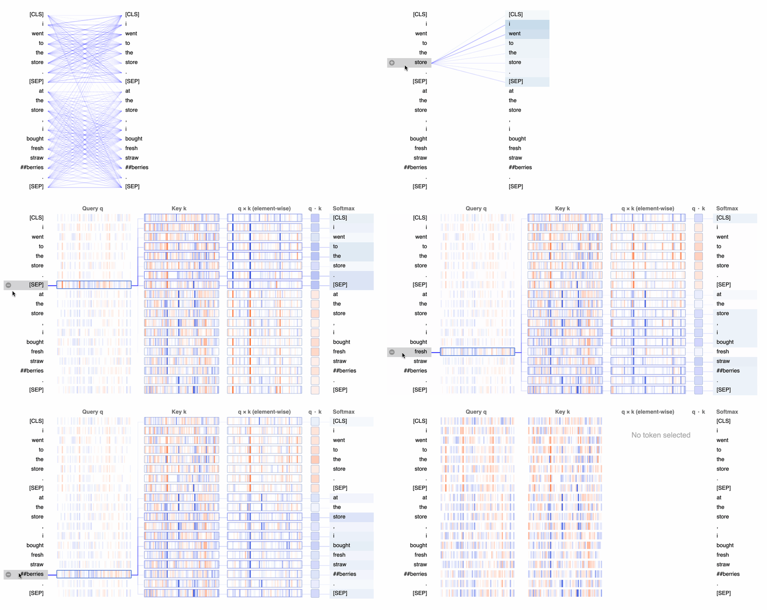
A useful visual explainer can be seen with the BERTViz tool [8] (see Figure 1.5) where we can observe attention for one or more attention heads in the same layer as well as how individual neurons in the query and key vectors are activated in the attention computation.
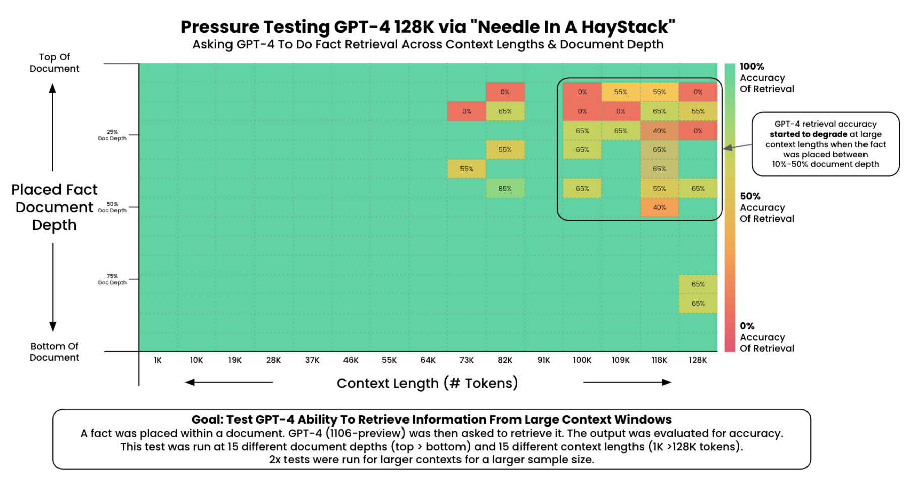
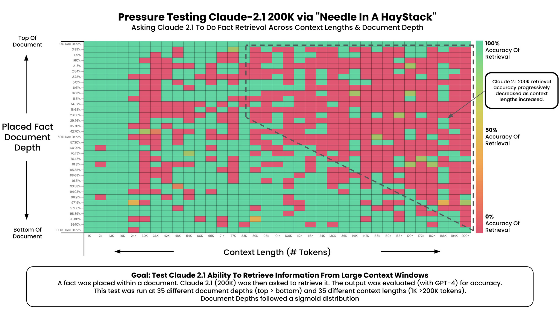
We can observe in the following experiments in Figure 1.6 that GPT4’s recall performance starts to degrade above 73K tokens where we observce low recall performance when fact is placed between 7-50% document depth. However, facts at the beginning of documents were recalled regardless of document length. This also seems to be the case for Anthropic’s Claude 2.1 model.
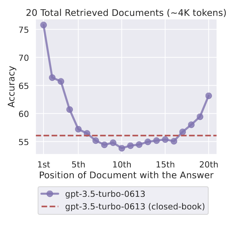
Transformers suffer from the “lost in the middle” issue with long contexts where the model struggles to retrieve the answer if the context is in the middle of the document. This is mitigated by prompt compression techniques which involve training smaller prompt compression LLMs to identify and remove non-essential tokens before feeding them to the larger LLM and retrieval-augmented-retrieval (RAG) techniques which involve adding additional context to prompts to allow LLMs to operate on facts fetched from external sources outside of LLM’s trained context. However, this involves relying on techniques and architectures to augment the input and output to the model as opposed to improving long context performance of the model itself.
1.1.1 Limitations of the the KV Cache
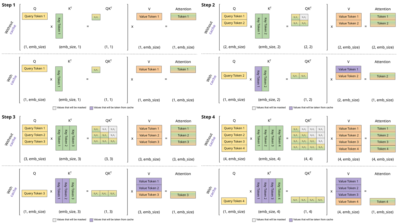
The KV cache is the caching of each key and value tensor of size d_head for each attention heads of each layer for each token in a batched sequence to enable the self-attention mechanism to scale linearly instead of quadratically. The precise space required by each tensor parameter will depend on the precision \(p_{a}\) (eg. 4bytes/parameter for full precision float32, 2 bytes/parameter for half-precision float16, 1 bytes/parameter int8) [11]. This can be expressed as:
\[ 2 \cdot BS \cdot T \cdot n_{layers} \cdot n_{heads} \cdot d_{head} \cdot p_{a} \tag{1.2}\]
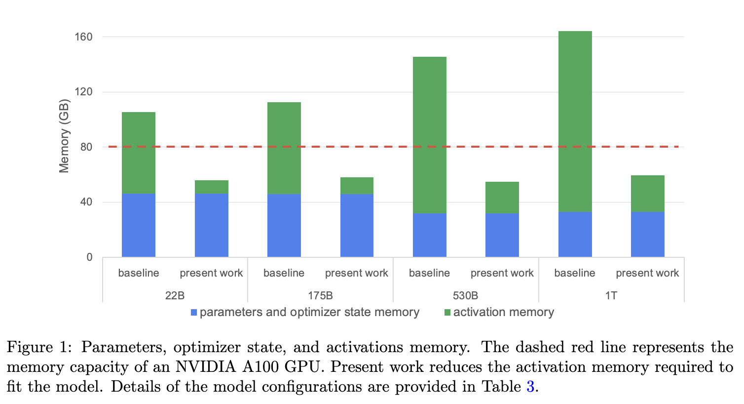
The challenge with the KV cache is that it will grow linearly with the sequence length and batch size. Since sequence length is unknown prior, the KV cache size can consume an unbounded amount of GPU memory in the order of ~1MB/token and can easily grow larger than the model weights if implemented naively. This is not to mention the amount of data transfer required to transfer the model and KV cache at scale. If we can reduce the GPU memory requirement to allow for more compute space, latency can be greatly improved.
There has been a lot of recent advancement in techniques and significant engineering efforts to reduce the KV cache for ever-growing context size. However, if we can try to solve this at the modelling level, it will greatly reduce the system complexity require to scale AI adoption in future. These techniques include [13]:
- novel attention architectures to reduce the number of attention heads
- cache compression strategies to more intelligently prioritise a fixed KV cache eg. caching the very first positional tokens (”sink tokens”) and the last neighboring tokens (local attention)
- efficient memory management to share the cache across different requests on the host especially for common tokens
- quantising the model weights and activations to reduce the GPU memory footprint
- storage capacity expansion such as offloading memory to CPU or single and multi-host model parallelism, a technique to pool memory over multiple devices by sharding the model over multiple GPUs used often when LLM cannot fit on single GPU in training
\(N\): Sequence length \(d\): Model parameters
| Pros | Cons |
|---|---|
| Unreasonably effective at modelling complex dependencies: Each token explicitly attends to all other tokens in the sequence. Unlike architectures that rely on a fixed-sized state as a summary, masked attention in transformers enables each token to see an uncompressed view of the sequence during training. | Quadratic scaling with context length: Since every input attends to all prior inputs, the total amount of computation increases quadratically both in time and space - \(O(N^2d)\). The cost of inference is therefore quadratic in nature, having to recalculate attention for the full sequence. However, this can be reduced to space and time complexity to \(\approx O(Nd)\) with a KV cache[14]. |
| Highly parallel training: There are no dependencies along the time dimension, and the core operations are matrix multiplications, which hardware accelerators have been excellent at parallelisation for decades. | Weak inductive bias: Unlike CNNs, there is almost no prior knowledge of dependency patterns. For example, position information only comes from absolute/relative positional embeddings. |
1.2 Limitations of RNNs for Long Contexts
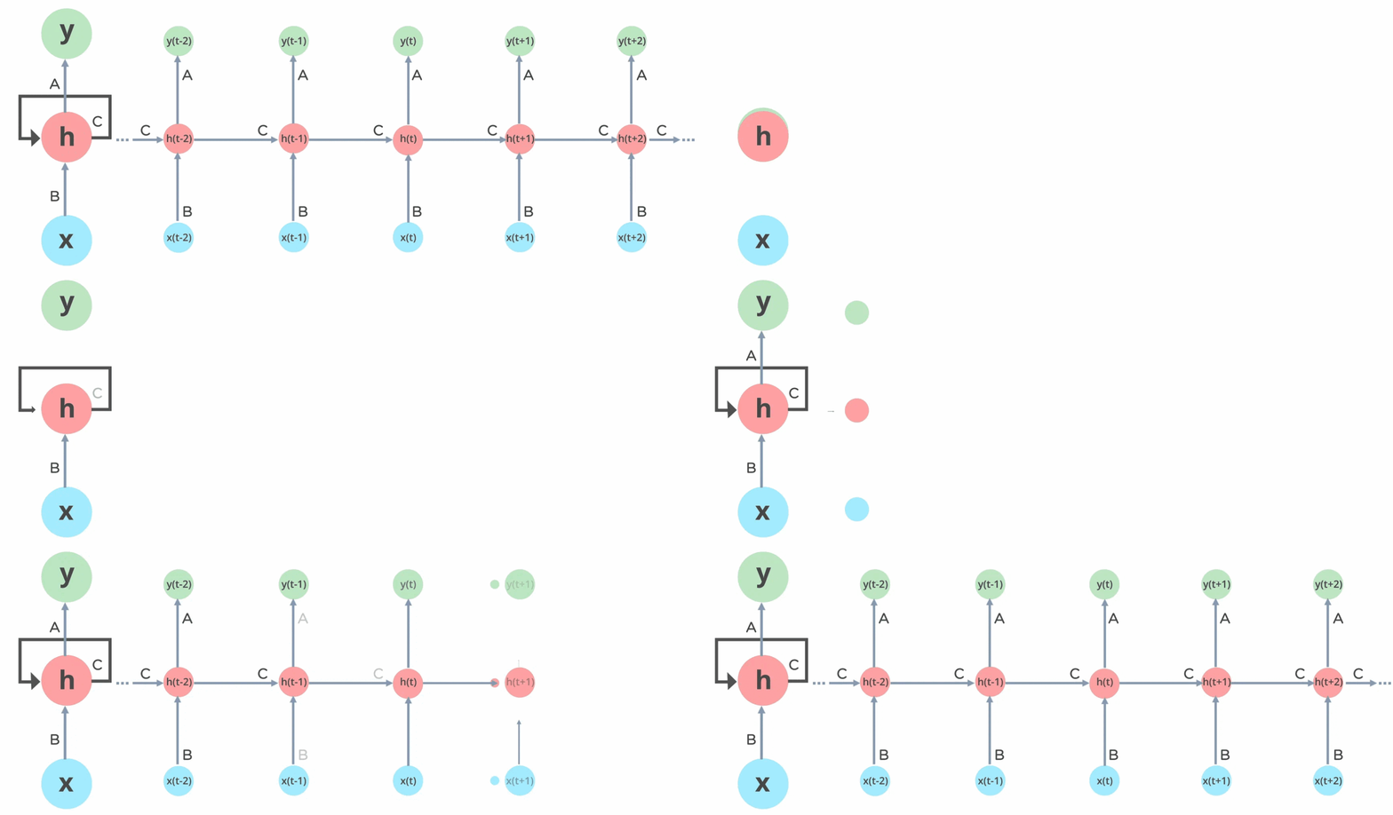
Before transformers, RNNs were the go-to architecture for sequence modeling where they process sequences iteratively, maintaining a hidden state that captures previous information. The fixed size state \(h_{t−1}\) represents all prior context in a sequence at time \(t\). However, RNNs suffer from vanishing and exploding gradient problems as the sequence length grows, making it difficult for them to learn long-range dependencies effectively. Additionally, the recurrent nature of RNN’s inhibit ability to parallelise training.
\[ \begin{align} & h_t &= \tanh(W_{hh} h_{t-1} + W_{xh} x_t) \\ & y_t &= W_{hy} h_t \end{align} \tag{1.3}\]
\(N\): Sequence length \(d\): Model parameters
| Pros | Cons |
|---|---|
| Efficient autoregressive inference: Since the hidden state \(h(t)\) encapsulates prior inputs, the model only needs to consider a small and constant set of new information for each subsequent input. | Ineffective modeling of complex dependencies: All prior context must be compressed, via static updates, into a fixed amount of bits. Therefore, RNNs often suffer with the vanishing gradient problem with long range sequences. |
| No limits to context length: There is nothing in the formulation that explicitly constrains the model to a maximal sequence length and therefore the state is constant. Inference scales linearly with sequence length. | Slow training: Training requires sequential backpropagation through time, making poor utilisation of hardware accelerators, e.g., GPUs. In feed-forward propagation and backpropagation, the computation of each state is contingent upon the previous step, therefore the training complexity is \(O(Nd^2)\). |
1.3 Complexity
In summary, the state space models are the only models with linear time and space complexity for both training and inference.
\(N\): Sequence length \(d\): Model parameters
| Aspect | RNNs | Transformers | State Space Models (SSMs) (Mamba) |
|---|---|---|---|
| Training Time Complexity | \(O(N \cdot d^2)\) | \(O(N^2 \cdot d)\) | \(O(N \cdot d)\) |
| Training Space Complexity | \(O(N \cdot d)\) | \(O(N^2 \cdot d)\) | \(O(N \cdot d)\) |
| Inference Time Complexity | \(O(N \cdot d^2)\) | \(O(N^2 \cdot d)\) without KV cache \(O(N \cdot d)\) with KV cache | \(O(N \cdot d)\) |
| Inference Space Complexity | \(O(d)\) | \(O(N^2 \cdot d)\) without KV cache \(O(N \cdot d)\) with KV cache | \(O(d)\) |
2 What are Structured State Space Sequence Models (S4)?
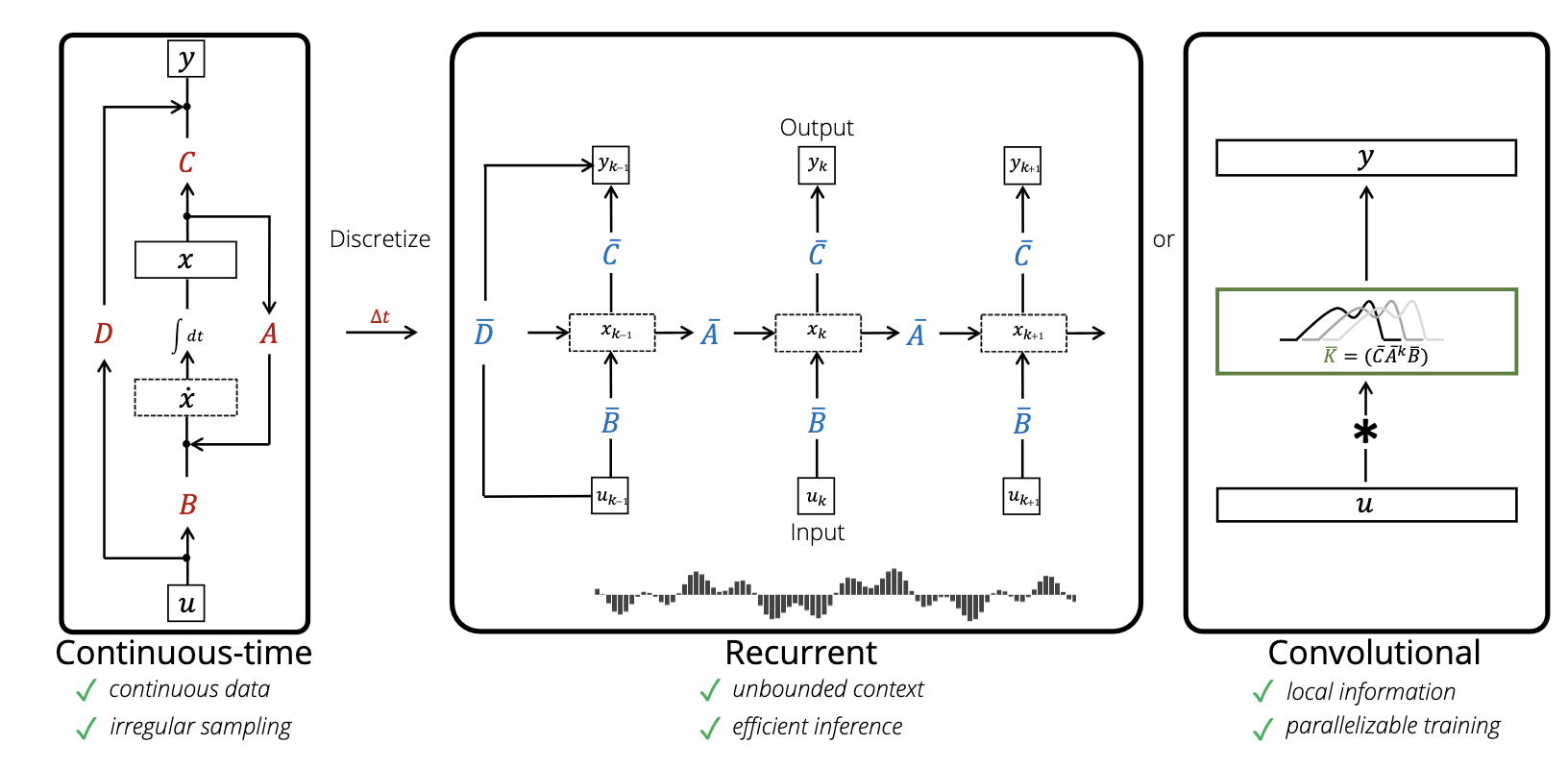
Structured state space sequence models (S4) are introduced as a unified framework for applying SSMs to sequence modelling and can be placed on a spectrum between highly compressed (e.g. RNNs) to highly explicit (e.g. transformers) based on their approach to information representation. Their architecture can be interpreted as a combination of recurrent, convolutional and continuous-time models with linear state-space layers [15] with online memory approximation in the form of the HIPPO matrix operator [5] to effectively approximate sequences with long-range dependencies. This framework allows us to represent the model in three representations; as an implicit continuous-time input signal, as a discretised recurrent network for efficient inference and as a convolutional representation which allows for efficient parallelisable training.
2.1 State Space Models
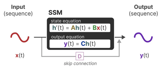
To understand S4, we must first understand their origins from classical SSMs, commonly used to describe state representations of continuous-time systems, mathematically formulated as a set of first-order differential equations. The state of the system is represented by a vector of variables \(x(t)\), and the dynamics of the system are described by how these state variables change over time (\(\mathbf{A}\)).
Therefore, at each timestep \(t\), we project the input sequence \(x(t) \in \mathbb{R}^{M}\) to higher-dimensional latent state space representation \(h(t) \in \mathbb{R}^{D}\) (memory state) to derive the predicted output sequence \(y(t) \in \mathbb{R}^{O}\).
\[ \text State \space equation: \quad h'(t) = \mathbf{A}h(t) + \mathbf{B}x(t) \tag{2.1}\]
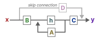
\[ \text Output \space equation: \quad y(t) = \mathbf{C}h(t) + \mathbf{D}x(t) \tag{2.2}\]
The matrices definitions therefore are:
- \(\mathbf{A} \in \mathbb{R}^{D \times D}\) the system matrix which describes the system dynamics (otherwise known as the state transition matrix)
- \(\mathbf{B} \in \mathbb{R}^{D \times M}\) the input matrix which describes how inputs affect the state
- \(\mathbf{C} \in \mathbb{R}^{O \times D}\) the output matrix which maps the state to the output
- \(\mathbf{D} \in \mathbb{R}^{O \times M}\) the feedthrough or direction transmission matrix which describes how the input directly influences the output
Often, we consider the the case of a single-input single-output system where \(O=M=1\) therefore \(\mathbf{D}=0\), where we omit \(\mathbf{D}x(t)\) by treating it as a skip connection.
These equations suggest that the SSM exhibits global awareness, as the current output is influenced by all preceding input data. When \(\mathbf{A}\), \(\mathbf{B}\), and \(\mathbf{C}\) have constant values, Equation 2.1 defines a linear time-invariant (LTI) system. Otherwise, it describes a linear time-varying (LTV) system, as in Mamba. LTI systems inherently lack the ability to perceive input content, whereas input-aware LTV systems are designed with this capability. This key distinction enables Mamba to surpass the limitations of S4.
2.2 Discretisation for Training and Inference
In order to apply the state space model to deep learning applications for language, audio, image data etc, we must first discretise the system. To achieve this, a timescale (step size) parameter, denoted as \(\Delta in \mathbb{R}\), is introduced to represent the resolution of the input to transform the continuous parameters (\(\Delta\), \(\mathbf{A}\), \(\mathbf{B}\)), into discrete forms (\(\mathbf{\bar{A}}\) and \(\mathbf{\bar{B}}\)).
There are many discretisation rules that can be applied to transform the parameters, in S4, they use the bilinear method. In Mamba, they apply the zero-order hold rule, we discretise the parameters as follows: \[ \begin{align} & \mathbf{\bar{A}} = \exp(\Delta \mathbf{A}) \\ & \mathbf{\bar{B}} = (\Delta \mathbf{A})^{-1} (\bar{\mathbf{A}} - \mathbf{I}) (\Delta \mathbf{B}) \\ & \approx (\Delta \mathbf{A})^{-1} (\Delta \mathbf{A})(\Delta \mathbf{B}) \\ & = \Delta \mathbf{B}. \end{align} \tag{2.3}\]
Thus, we transform the continuous signal-to-signal problem \(x(t)\rightarrow y(t)\) to a discrete sequence-to-sequence problem \(x_k \rightarrow y_k\), by holding the input constant over each interval and applying the ZOH rule, which can be then computed as a linear recurrence similarly to RNNs Equation 1.3. This discretised recurrent form is used for efficient autoregressive inference where the inputs are seen one timestep at a time (see Figure 1.9), especially for systems where \(\Delta t\) is small. In practice, \(x_k\) is a feature vector of size \(\mathbf{C}\).
From Continuous to Discrete SSMs With the Zero Order Hold Rule
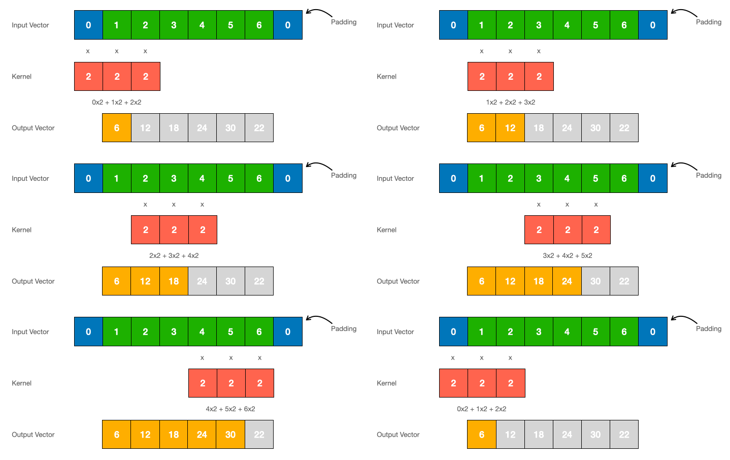
To acommodate for parallelised training, we can unroll the linear recurrent form to yield a global convolutional representation to Equation 2.4
\[ y = x * \mathbf{\bar{K}} \tag{2.4}\]
where \(\mathbf{\bar{K}}=(\mathbf{C}\mathbf{\bar{B}}, \mathbf{C}\mathbf{\bar{A}}\mathbf{\bar{B}, ..., \mathbf{C}\mathbf{\bar{A}}}^{T-1}\mathbf{\bar{B}})\) represents the SSM convolutional kernel with length \(T\) of the entire sequence. We can do this because \(\mathbf{\bar{A}}\), \(\mathbf{\bar{B}}\), and \(\mathbf{C}\) are constant. To compute this efficiently, we apply the discrete convolution theorem trick which states that the convolution of two sequences can be computed as the inverse FFT of the product of their FFTs, transforming the convolution operation into a multiplication in the frequency domain.
2.3 The State Transition Matrix \(\mathbf{\bar{A}}\)
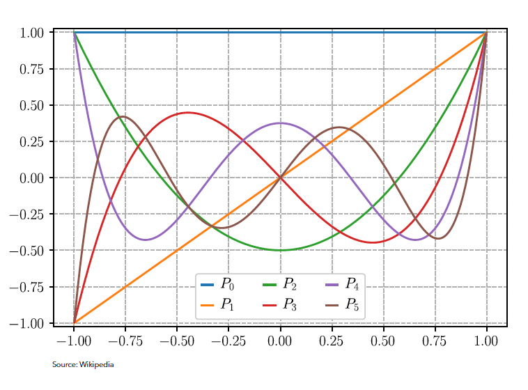
The core idea that makes S4 work is the theory of treating memory as an online polynomial function approximation problem where a function \(f(t): \mathbb{R} \rightarrow \mathbb{R}_{+}\) can be summarised by the summation of its optimal coefficients in terms of orthogonal polynomial basis functions. This led to the authors, Gu et al, to introducing the HIPPO (high-order polynomial projection operators) matrix operator [5] applying Legendre polynomials for signal decomposition for continuous-time memorisation. Their orthogonal nature ensures minimal redundancy and interference between different components, leading to stable and efficient representations of sequences with the ability to represent functions between an interval \([1, -1]\).
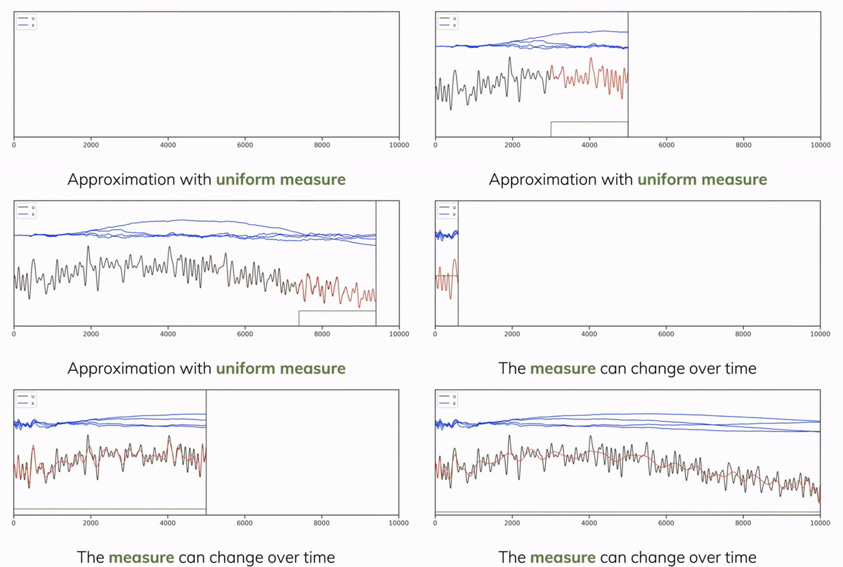
This state transition matrix aims to compress the past history into hidden state that has enough information to approximately reconstruct the history in a lower-dimensional state of fixed memory size. We can see in Figure 2.5 how we can learn the compressed form \(y(t)\) of the input signal \(u(t)\) as a linear combination of the Legendre polynomials in \(x(t)\) (or \(h(t)\) from our notation above) by applying the HIPPO matrix as \(\mathbf{\bar{A}}\) at each timestep.
In order to compute this matrix even more efficiently, since we have a structured matrix with known properties, we can speed up the computation of \(\mathbf{\bar{K}}\) significantly, and overcome the \(O(Td^2)\) computational complexity and \(O(Td)\) space complexity in applying \(\mathbf{\bar{A}}\) for each time step in the sequence.
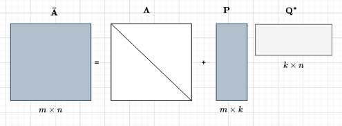
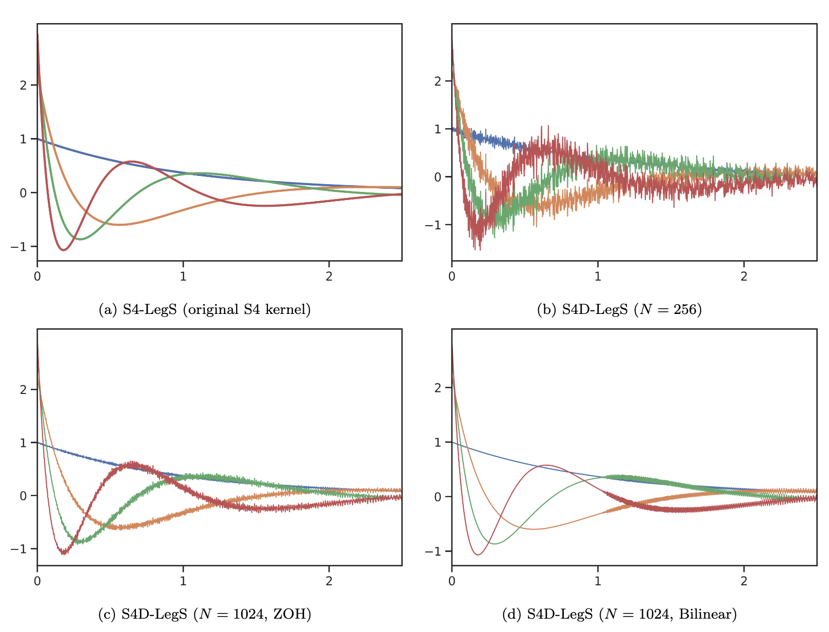
The original S4 approach was to leverage the Diagonal Plus Low-Rank (DPLR) structure in complex space [19] which significantly reduces the space and time complexity as we only need to store and compute the diagonal elements and low-rank components of the dense matrix. It can be expressed as \(\mathbf{\bar{A}}=\mathbf{\Lambda}+ \mathbf{PQ^*}\) where \(\mathbf{\Lambda}\) is the diagonal matrix and \(\mathbf{PQ}\) are low-rank matrices (vectors for rank-1 updates). The addition of the low-rank term allows the DPLR matrix to capture more complex relationships in LRD compared to a simple diagonal matrix whilst specialised techniques like the Woodbury identity make operations on DPLR matrices feasible and efficient. This was followed by a paper that showed empirically that just using the diagonal matrix and removing the low-rank portion of the DPLR form of the HIPPO matrix, yielded similar results [19].
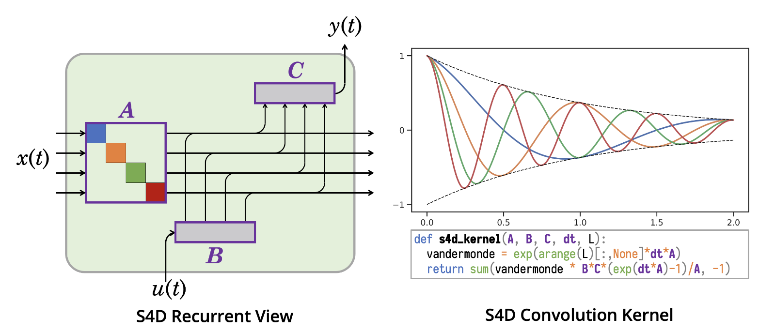
This work led to S4D used in Mamba [20], further improving the computational effiency and expressiveness of \(\mathbf{\bar{A}}\) by leveraging the Vandermonde Matrix to compute the diagonal matrix, leveraging the properties of eigenvectors and eigenvalues to efficiently capture more complex relationships between state variables (such as powers and exponentials). This is expressed as \(\mathbf{\bar{A}}=\mathbf{V \Lambda V^{-1}}\) where \(\mathbf{\Lambda}\) is the diagonal matrix of eigenvalues, \(\mathbf{V}\) is the Vandermonde matrix of eigenvectors and \(\mathbf{V^{-1}}\) is the inverse Vandermonde matrix.
3 How does Mamba improve on S4 to be a potential alternative to transformers?
There are several core architectural improvements that Mamba introduces to perform competitively with transformers to overcome S4 weaknesses on tasks that are vital to language modelling and generation enabled by dynamic nature of attention. Namely, the ability to perform context-aware reasoning as \(\mathbf{\Delta}\), \(\mathbf{A}\), \(\mathbf{B}\), and \(\mathbf{C}\) are constant for each input, meaning they cannot “attend” to parts of the sequence or selectively retain information based on the input.
In order for the SSM model to selectively retain information, the system is made time-variant eg. \(\mathbf{\Delta}\), \(\mathbf{\bar{B}}\), and \(\mathbf{\bar{C}}\) are now functions of input \(x(t)\), where \(\mathbf{\bar{A}}\) also depends on the input through \(\mathbf{\Delta}\) (\(\mathbf{\bar{A}} \rightarrow \mathbf{\bar{A}}_{\theta (x)}\)). Since the time step \(\mathbf{\Delta}\) is now learnable, \(\mathbf{\Delta}\) is roughly proportional to the size of the state update; the model will learn to focus on the input tokens and update the state that correspond to large values of \(\mathbf{\Delta}\), and ignore input for when \(\mathbf{\Delta}\) is small whilst persisting the state.
3.1 Selective SSM for Context Aware Reasoning
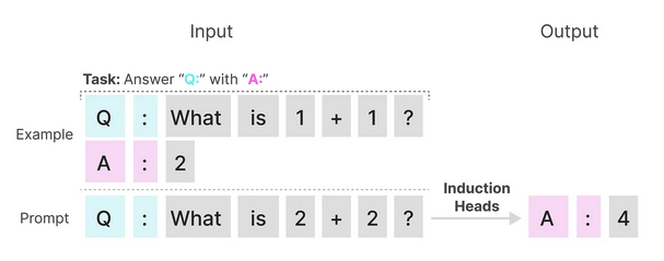
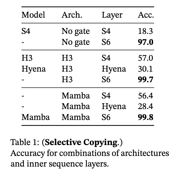
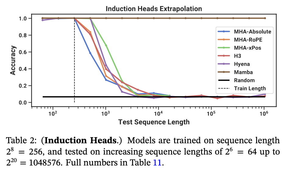
A model’s ability to perform in-context reasoning can be inferred from their performance on the tasks of selective copying and inductive reasoning [3]. Selective copying refers to the model’s ability to identify and reproduce specific phrases, entities or patterns in the input, and incorporate it appropriately in the generated output and is a task to test a model’s memorisation capabilities. Induction heads is an associative recall task to test a model’s ablility to perform inductive reasoning based on observed patterns, and learned underlying concepts and relationships.
This introduction of selection enables Mamba to perform:
- over 2x as well than S4 and predecessor models on the selective copying task reaching accuracy over 97%.
- ~100% accuracy on inductive heads due to ability to selectively remember the relevant token while ignoring everything else in between. It is able to generalise to million-length sequences, 4000x longer seen during training, whilst other methods such as multi-head attention (MHA) variants fail to perform at 2x sequence length.
3.2 Selective SSM Layer for Parallelised Training
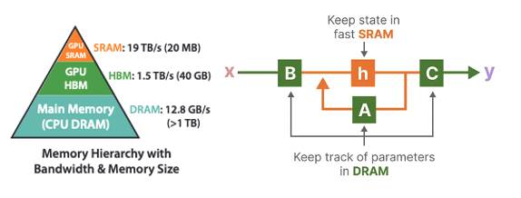
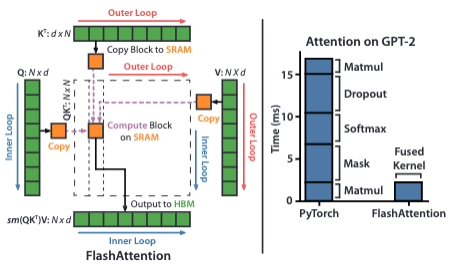
However, making the system time-varying means we can no longer perform convolution in Equation 2.4 to parallelise training since it assumes a fixed kernel. To address this, Mamba introduces the selective scan layer. It is the implementation of a hard-aware selective parallel scan algorithm with the same GPU kernel fusion techniques in FlashAttention [21] for transformers, as a result of Mamba being a collaborative paper between Albert Gu (S4) and Tri Dao (FlashAttention). Therefore, the core optimisations for all three techniques, parallel scan, kernel fusion and recomputation in the selective SSM layer are to try and perform as many operations in the fast memory (SRAM) layer of the GPU before saving results back to high-bandwidth memory (HBM) (see Figure 3.6). This reduces the data transfer (IO) between them, as loading is often the slowest process [22]. For more details on model optimisation on GPUs, this is a good read from first principles.
3.2.1 Parallel Associative Scan
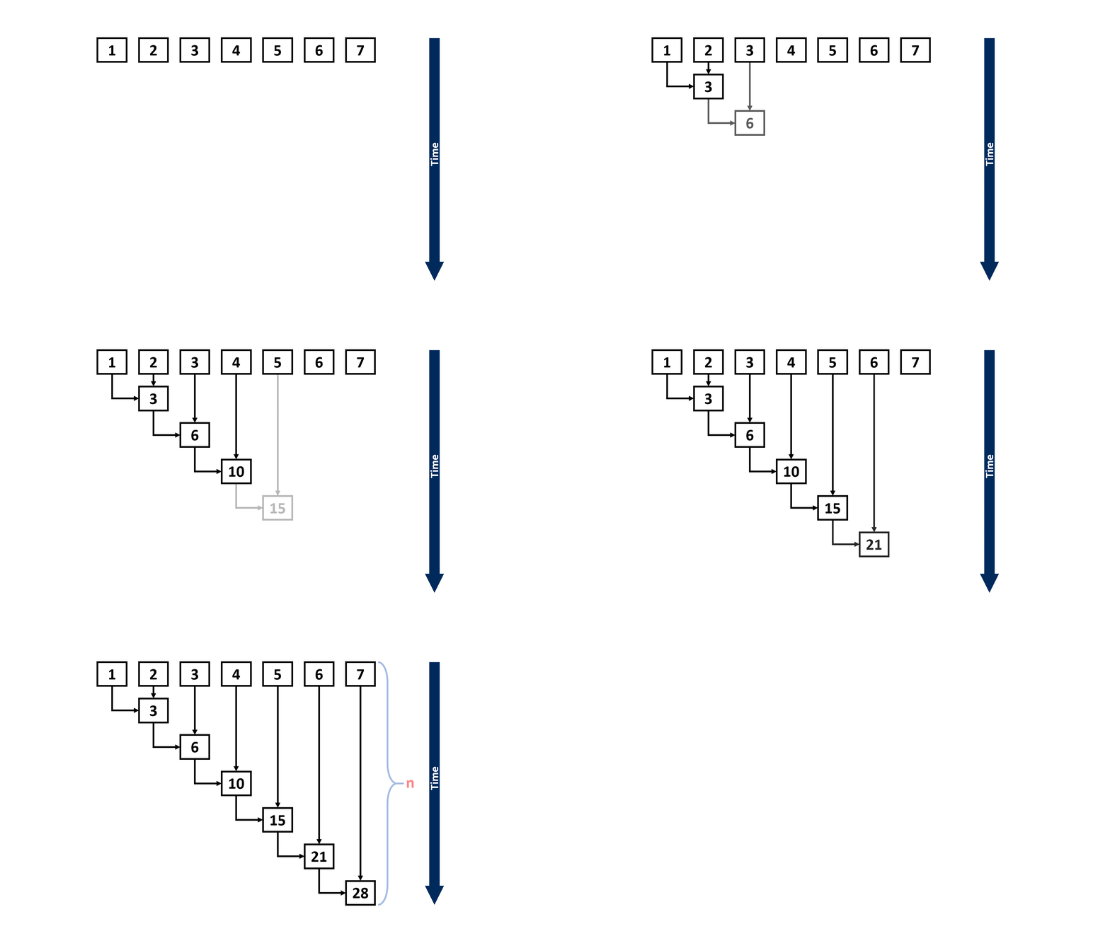
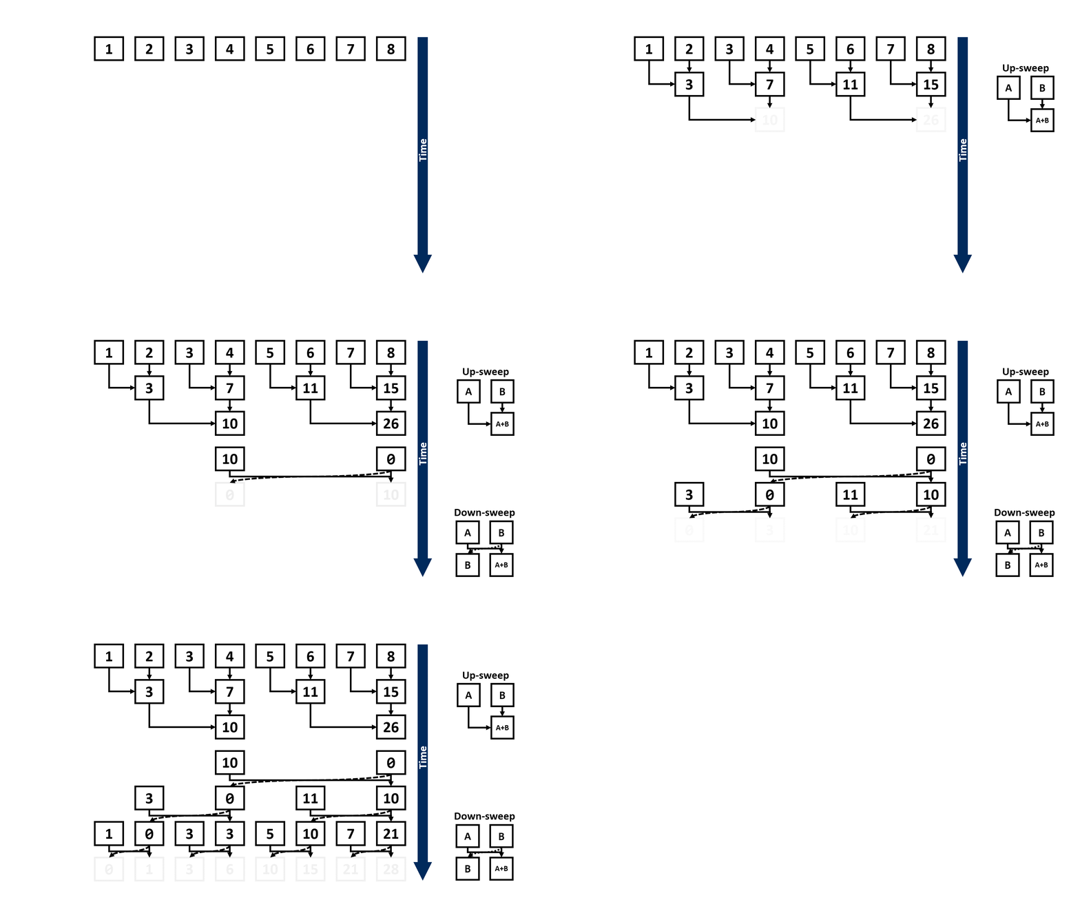
Despite not being able to parallelise the state computation with convolution, we can speed up the recurrent computation with the parallel associative scan, otherwise known as the parallel prefix sum (scan) problem. The work-efficient parallel prefix scan algorithm is also known as the Blelloch Algorithm named after it’s author. The recurrent formula of the SSM model can also be thought of as a scan operation where each state is the sum of the previous state and the current input. To generate the output, we multiply each \(h_k\) with \(C\) to generate \(y_k\). The parallel scan algorithm is based on the associative property where \(A * B * C = (A * B) * C = A * (B * C)\) which states that the order of the operations does not matter therefore reducing time complexity from \(O(N)\) to \(O(N/pt)\) where \(pt\) is the number of parallel threads on GPU. See here for more implementation details of the parallel scan operation and deeper understanding of the binary associative operator in parallelising computation of \(h_k = \mathbf{\bar{A}}h_{k-1} + \mathbf{\bar{B}}x_k\).
3.2.2 Kernel Fusion
One of the biggest efficiency gains is from implementing the parallel associative scan as a single GPU kernel operation through GPU kernel fusion. The discretisation, parallel associative scan operation and multiplication with \(\mathbf{C}\) are performed in the SRAM before writing results back to HBM. Therefore, a lot of time is saved by creating a custom kernel to fuse the operations required to perform the scan operation into a single layer to reduce the IO between SRAM and HBM by factor of \(O(D)\) - the state dimension [3]. When the sequence length \(T\) is too long to fit the full sequence into SRAM which is much smaller than HBM, the sequences are split into chunks where the fused scan is performed on each chunk.
3.2.3 Recomputation
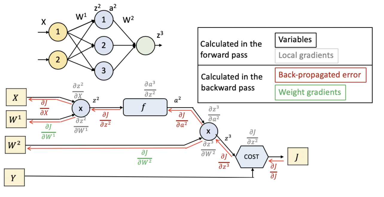
The memory and compute requirement is further optimised by re-computing cheap operations instead of saving and reading intermediate states between stages in the entire selective SSM block (input projection, convolution, activation, scan, output projection). For instance, re-computing intermediate states (\(\mathbf{\Delta}\), \(\mathbf{\bar{A}}\), \(\mathbf{\bar{B}}\), \(\mathbf{\bar{C}}\)) to compute gradients on the backward pass vs reading them from HBM memory from the forward pass.
3.3 Mamba Architecture
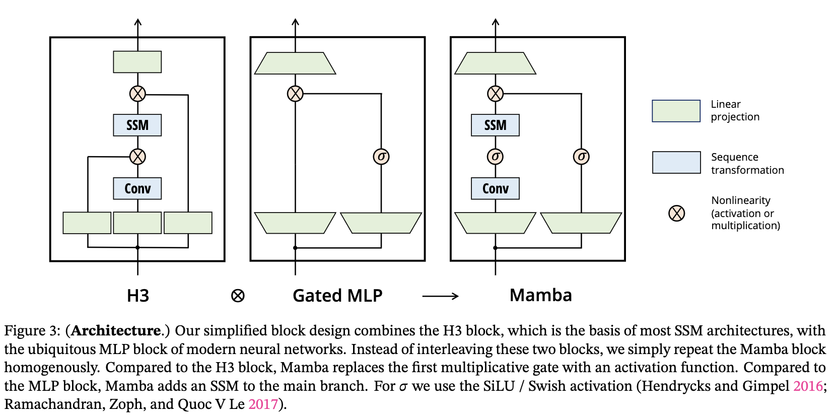
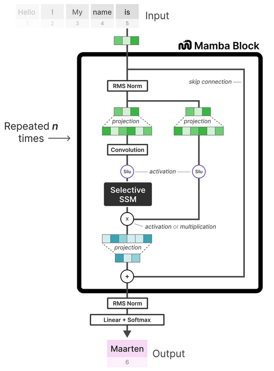
The Mamba model is made by stacking multiple layers of Mamba blocks, similar to self-attention in the transformer. It is heavily inspired by its predecessor, the Hungry Hungry Hippo (H3) Architecture [25]. It starts with projecting inputs to hidden state, followed by convolution over projected dimensions with sigmoid-weighted linear unit (SILU) /Swish activation [26]. The SSM operation is then computed followed by the skip connection operation \(\mathbf{D}\) before downscaling for another linear projection.
The full architecture includes tokenising inputs to an embedding later, followed by the Mamba block repeated N times for the length of the sequence N with the inclusion of couple RMS Norm normalisation layers and a softmax layer for choosing the next output token.
3.4 Mamba vs LLMs Performance for Language Modelling
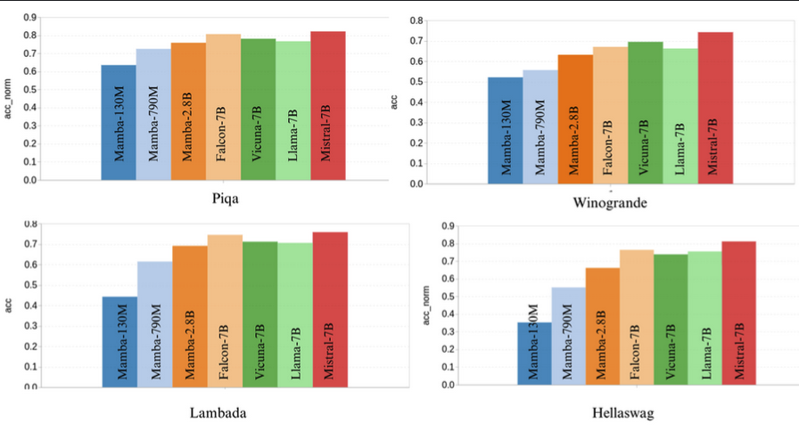
Mamba has shown extremely promising results compared to transformer LLM models, where it has been shown that it has been able to perform competitively on commonsense reasoning benchmarks with models twice their size (eg. Mamba 2.8B vs Mixtral 7B). However, large-scale research on Mamba vs transformer models of the same size is yet to be conducted. Their prevalence is yet to be seen given the industry’s investment into productionisation of transformer-based architectures.
4 Conclusion and Future Directions
Mamba therefore introduces a promising alternative to transformers as a general sequence model backbone for building foundation models for different domains and modalities such as signal data, genomics, audio, video and large text corpuses. It’s selection mechanism for SSM models enables efficient and effective state representation, enabling context-aware reasoning on large contexts, with linear scaling with sequence length. This enables us to perform in-context reasoning with much longer context windows to overcome the short-term memory limitations of transformers.
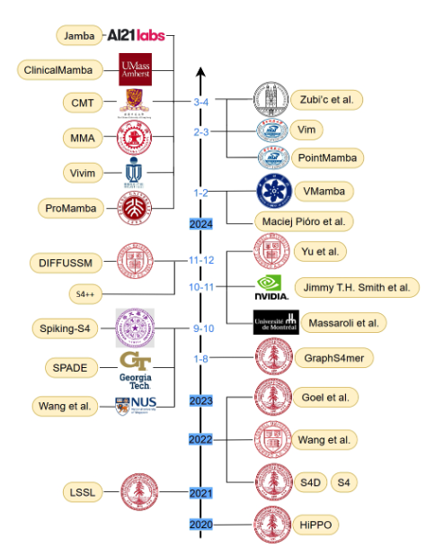
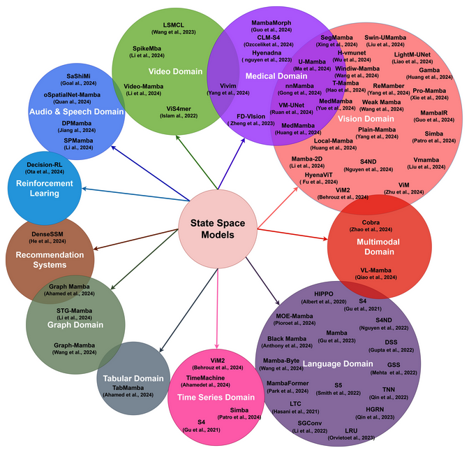
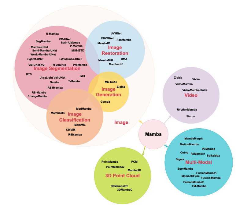
Since then, there has been a plethora of Mamba variants in multiple mediums and domains working to push and evaluate the performance potential as well as highlight challenges and limitations of the SSM architecture in coming years. In summary, current SSM models have yet to reach the level, scale, maturity and performance of transformer networks as a general backbone architecture, but the lowered GPU consumption is worth further exploration and research as we reach scaling limits.
4.1 Applications and Architectures
From a recent survey, there are still stability challenges scaling SSMs to the same network size as SoTA transformers especially in vision [27]. Fusion techniques may fill in each others’ shortcomings between CNNs, vision transformers and vision mamba models in future to allow for better generalisation performance with long-context dependencies. For example, this has lead to the open-source release of a new LLM foundation model, Jamba, from AI32 Labs fusing the Transformer, Mamba, and MoE (Mixture-of-Experts) architectures to enable context length of 256K tokens with performance reaching Mixtral-7B and Llama2-7B with a reduced KV cache memory footprint of only 4GB [29].
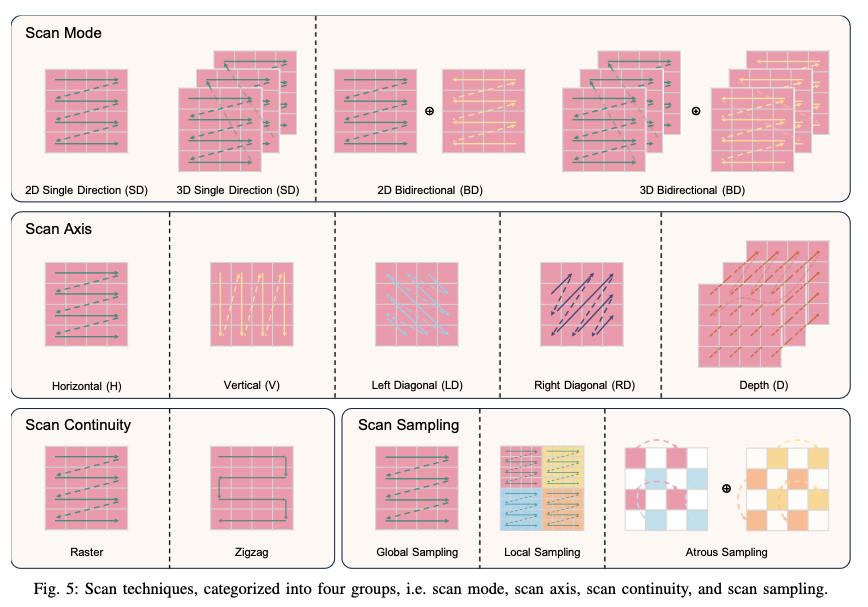
The plethora of Mamba vision variants of late extend the selective scan algorithm to 2 dimensions where the scan techniques can be categorised into four groups: scan mode, scan axis, scan continuity and scan sampling (see Figure 4.2).
However, a recent paper, MambaOut, highlights that Mamba models may not be needed for tasks that do not require long-sequence dependencies and autoregressive characteristics, such as image classification [30] which they prove by showing that MambaOut can outperform SoTA vision Mamba models on ImageNet-1K classification without the Mamba block. It will be fruitful, however, to evaluate Mamba’s performance on detection and segmentation in long-context settings such as with long-term video sequences (movies) or high-dimensional imagery (remote sensing).
Modifying Mamba’s inherent 1D nature of selective scan meant for a causal sequential stream to a bi-directional 2D scan technique has posed algorithmic challenges in scalability and stability, as well as maintaining spatial information without redundancy in computation. Therefore, there needs to be advancements in the scanning operators in order to apply Mamba on higher-dimensional non-causal visual data more effectively in future and to capture and obtain more comprehensive skewed feature representations to enhance the feature learning in SSMs.
Please feel free to suggest any improvements or corrections. Thanks for reading and hope you learnt something useful from my journey! :)
5 References
This primer is a consolidation of bits and pieces in the following list. Feel free to dig further below!




![Discrete SSM Diagram [1]](./discrete_ssm.png)
